Antenna patterns & the sensor panel

By default Waveshed models an isotropic antenna with equal gain in every direction. Real transmitters are rarely isotropic, so RF mode has an advanced Sensor / Antenna panel where you can shape the antenna, see it as polar plots, and save or load it. Here is what every control means.

1. Power: ERP, or transmitter power + gain

The Power field defaults to ERP, the Effective Radiated Power in watts, referenced to a half-wave dipole. The engine converts it to EIRP internally by adding 2.15 dB (the dipole’s gain over isotropic), then subtracts path loss to get the received signal.

Switch the Power control to TX + Gain when you know the transmitter and antenna separately. Enter the transmitter power in watts and the antenna peak gain in dBi, and Waveshed folds them into the same ERP (ERP = TX power + gain minus 2.15 dB). Either way you are describing the energy actually radiated. Gain belongs here, with the power, not on the pattern.

2. Open the Sensor / Antenna panel

Switch to RF Propagation, then expand Sensor / Antenna (advanced) below the RF parameters. Pick a pattern type and the relevant controls appear.

3. Choose and shape a pattern

Five generators cover most antennas, plus a custom mode for imported patterns:

• Isotropic, omnidirectional, 0 dBi, the engine default.
• Dipole (λ/2), omnidirectional in azimuth with the classic doughnut elevation shape (nulls overhead).
• Directional, a Yagi/parabolic main lobe with a back lobe. Set beamwidth, front/back ratio and sidelobe floor.
• Sector, a flat-topped wedge of a chosen width, like a base-station panel.
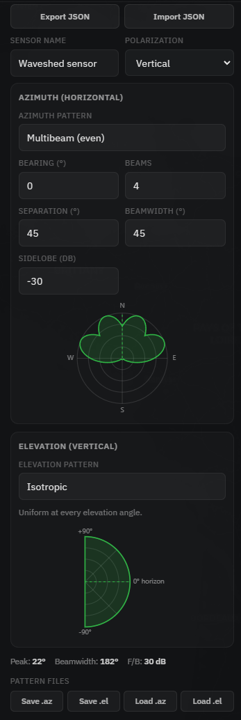
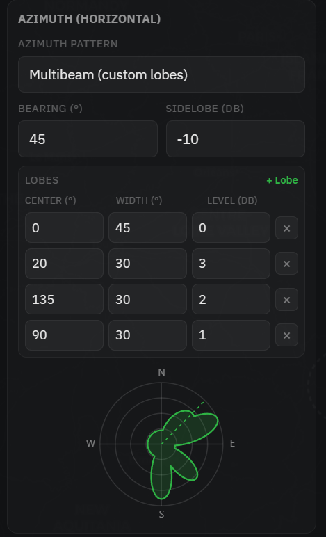
• Multibeam, any shape built from a list of lobes, each with its own centre, width and gain.

Bearing points the main beam (° from True North), and Down-tilt tilts it below the horizon. The readout under the plots shows the peak direction, the −3 dB beamwidth and the front/back ratio. Hover any label for a one-line explanation.

4. What the pattern contains

A pattern is two unitless shape tables. Azimuth: 361 points, 0–360° clockwise from True North. Elevation: 181 points, −90° (down) through 0° (horizon) to +90° (up). Each value is a linear gain from 0 to 1, where 1 is the peak. The engine applies them as 20·log₁₀(gain) and multiplies azimuth by elevation, so a value of 1 means no loss and 0.5 means −6 dB. The peak (1.0) is the main-beam gain you set in the Power field. The table only steers it.

5. Import, export & .az/.el

Export JSON saves the whole sensor (location, height, frequency, ERP, polarization and both patterns) as a single file. The parameter and pattern blocks match the MPT SIGMA emitter format, so the file moves between tools. Import JSON reads it back. Importing an MPT SIGMA emitter works too.

You can also Save or Load individual SPLAT! NG / AETHER .az and .el files. On import the header line is read, so the antenna bearing (.az) and mechanical tilt (.el) come across and are shown, not discarded.

6. How the pattern shapes coverage

In the browser preview the horizontal (azimuth) pattern is applied to the coverage map, so a directional antenna immediately carves a beam out of the circle. The AETHER engine applies the full azimuth × elevation pattern from the saved sensor config. Either way, the math is the same one the RF coverage workflow uses.